
DS City is known for its fine meats, but no company makes better sausages and roasts than The Roast Busters. They have come to you to seek your help on a seemingly easy task that is part of any introductory lesson in operations research: a simple production planning problem with two products and two side constraints. Surely you can do that, can't you?
The Roast Busters only make two products: sausages (S) and roasts (R). They employ five skilled workers who each work 4 hours per day on meat preparation and can produce a sausage with a hands-on effort of 1 minute and 12 seconds and a roast with 8 minutes of manual labor. They also have 25 "Sloth Pots" which are their secret to producing the most tender meats. The Sloth Pots run 24 hours per day. A sausage needs to slow-cook in a Sloth Pot for 24 minutes, a roast for 288 minutes (yes, they follow their recipes this precisely!).
You note down the side constraints for your optimization:
- 72 Q_S + 480 Q_R <= 72,000
- 24 Q_S + 288 Q_R <= 36,000
- Q_S, Q_R >= 0
where Q_S is the number of sausages produced and Q_R is the number of roasts. So simple, just as in the very first OR course you took! Your ship starts to sink when you ask about the corresponding profits and maximal demands.
"Those are for you to figure out!" the Roast Busters tell you. You have to set the prices. The cost to produce a sausage is $1.30, and the cost of a roast is $6.00. We also know about the price sensitivity of Roast Busters customers (P_S is the price in dollars for a sausage, P_R the price in dollars for a roast):
- Demand for sausages D_S = 6,000 - 1,500 * P_S
- Demand for roasts D_R = 160 - 4 * P_R
The only thing you spot is that the first side constraint means that we can never produce more than 1,000 sausages and that we should therefore never ask for less than $3.33 for a sausage. But how are you going to find the optimal prices and production quantities for both products?
________
Scroll down for a bonus question and the solution!

Bonus question for the truly stellar operations researchers: How would you set the prices and production quantities when the customer demand varies around the estimate following a normal distribution with a standard deviation of 10% of that estimate (where the variability is independent for each product)?
Scroll down for the solution!

When you only have access to a linear solver, a typical way to handle a problem like this is as follows: First, we determine the profit-maximizing prices for our products, taking only maximum production levels into account. We find that taking $3.33 for sausages and $23 for roasts is optimal (analytically minimize (160-4x)*(x-6) for the latter using the first and second derivations). We set up a linear program using these prices and the corresponding demands of 1,000 sausages and 68 roasts. The optimal production levels we then get are 546 sausages and 68 roasts. We finally hand these numbers to our revenue management department, which keeps the cost of roasts at $23 but increases the price of sausages to $3.63 without lowering the expected demand below the 546 sausages we said we were going to produce. Our total profit based on this common procedure is $2,428.18.
Rather than solving the problem piecemeal as above, a better way to get to a solution is by employing a non-linear solver like InsideOpt Seeker(TM).
Maximize T_S * P_S - Q_S * 1.30 + T_R * P_R - Q_R * 6
such that
- 72 Q_S + 480 Q_R <= 72,000
- 24 Q_S + 288 Q_R <= 36,000
- D_S = max(6,000 - 1,500 * P_S, 0)
- D_R = max(160 - 4 * P_R, 0)
- T_S = min(Q_S, D_S)
- T_R = min(Q_R, D_R)
- Q_S, Q_R, P_S, P_R >= 0
using the true sales variables T_S and T_R. This leads to prices P_S = $3.53 and P_R = $28.75 and production levels Q_S = 700 sausages and Q_R = 45 roasts. Our total profit is now $2584.75 per day, 6.45% more profit than the linear programming solution.
Not bad, but in reality our demands estimates come with some level of uncertainty. Traditional solvers fall short entirely as soon as our demand forecasts become stochastic. In the bonus question, the demands could vary normally with a standard deviation of 10% up or down from the demand estimate. For this case, InsideOpt Seeker(TM) suggests keeping the production levels the same (Q_S = 700 sausages and Q_R = 45 roasts) but lowering the prices slightly: P_S = $3.48 and P_R = $28.62. With these settings, Seeker assesses the expected profit to be $2,477.48—still a solid percent ahead of the solution of the linear programming approach when there is absolutely no variability in demand. However, there is variable demand, and the LP solution drops in expected profit to $2300.63 when the demand varies. That is 7.69% below the Seeker(TM) solution.
Can you really afford to continue using suboptimal optimizers?
For your interest, see the complete Seeker(TM) model for the stochastic bonus case below.
import seeker as skr

# Create a Seeker Environment
env = skr.Env("Seeker_Licence.sio", stochastic=True)
env.set_stochastic_parameters(round(1e6), 0)

# Create the Decision Variables
price = [env.ordinal(1, 400) / 100, env.ordinal(1, 4000) / 100]
quantity = [env.ordinal(0, 3000), env.ordinal(0, 300)]

# Add Constraints
env.enforce_leq(72 * quantity[0] + 480 * quantity[1], 72000)
env.enforce_leq(24 * quantity[0] + 288 * quantity[1], 36000)

# Derive Demand Values from the Prices
demand = [env.max_0(6000 - 1500 * price[0]), env.max_0(160 - 4 * price[1])]
noise = [env.normal(1, 0.1) for _ in range(2)]
unc_demand = [demand[i] * noise[i] for i in range(2)]
exp_demand = [env.aggregate_mean(unc_demand[i]) for i in range(2)]

# Compute the True Sales Numbers
sold = [env.min([unc_demand[i], quantity[i]]) for i in range(2)]

# Compute the Resulting Profit
cost = [1.3, 6]
profit = [sold[i] * price[i] - cost[i] * quantity[i] for i in range(2)]
exp_profit = [env.aggregate_mean(profit[i]) for i in range(2)]
exp_total_profit = env.sum(exp_profit)

# Optimize for 60 Seconds
env.maximize(exp_total_profit,  60)

# Extract the Solution
print("Expected Profit", exp_total_profit.get_value())
print("Price", [price[i].get_value() for i in range(2)])
print("Quantity", [quantity[i].get_value() for i in range(2)])
print("Demand", [demand[i].get_value() for i in range(2)])
print("Evaluations", env.get_number_evaluations())
This program creates the output:
Expected Profit 2477.4831316738547
Price [3.48, 28.62]
Quantity [700.0, 45.0]
Demand [780.0, 45.72]
Evaluations 217945
As usual, we can also visualize how this expected profit is distributed:
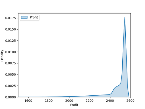
We can also ask Seeker(TM) what the likelihood of a profit lower than $2,000 is, which it assesses at 1.85%. If The Roast Busters are fearing a cash flow problem, we can also ask Seeker(TM) to, e.g., minimize the risk of ending up with less than $2,000 while enforcing that the total expected profit remains at least $2,400.
# Add Risk Term and Constrain Objective
risk = env.aggregate_relative_frequency_leq(2000, env.sum(profit))
env.enforce_geq(exp_total_profit, 2400)

# Optimize for 60 Seconds
env.minimize(risk,  60)
Expected Profit 2400.7260870068135
Price [3.33, 29.31]
Quantity [720.0, 42.0]
Demand [1005.0, 42.760000000000005]
Risk 0.001066

We note that Seeker(TM) lowers the price of sausages by about 5% but increases sausage production only mildly. By leaving a larger gap between production and expected demand, we obviously lower our opportunity, but we also run a lower risk of overproduction, which would cut into our profit. Overall, the risk of ending up with a profit lower than $2,000 is now down from 1.85% to 0.107%. That is a 17-fold reduction in risk, which costs us, on expectation, $77.
We built Seeker(TM) so that you can sculpt the risk profile of your operational plans to fit your business objectives. Please reach out to one of our specialists if you want to learn more about Seeker(TM). Or do you prefer butchering your business problems until your current solver can handle the pieces?